R Plot Gallery
Note: Don’t be fooled by the subtitle that tells you this article is a 1 min read.
In this post, I have listed plenty of plots generated by R. You can enjoy these plots as much as you like. If you are interested in how to reproduce these plots, please click on the Code button below the plots. If you are interested in what these plots can tell you, please click on the Explanation button next to Code. I hope you enjoy this gallery!
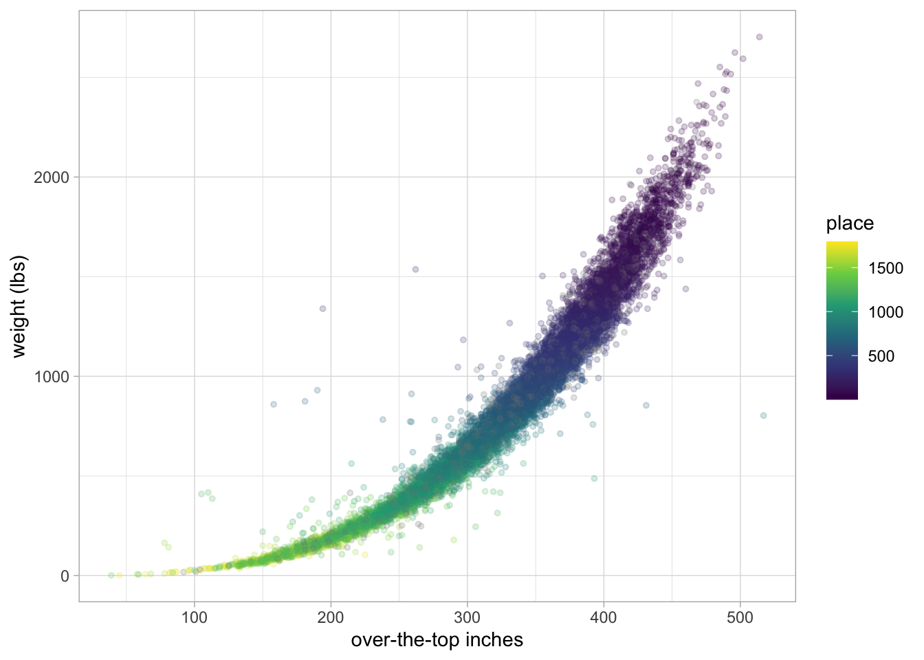
pumpkins %>%
  filter(ott > 20, ott < 1e3) %>%
  ggplot(aes(ott, weight_lbs, color = place)) +
  geom_point(alpha = 0.2, size = 1.1) +
  labs(x = "over-the-top inches", y = "weight (lbs)") +
scale_color_viridis_c()Already added to the schedule!
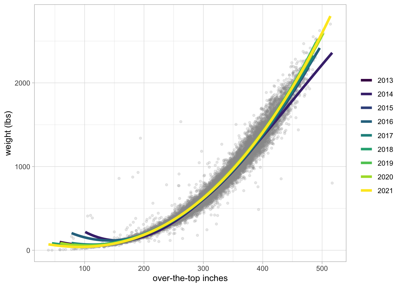
pumpkins %>%
  filter(ott > 20, ott < 1e3) %>%
  ggplot(aes(ott, weight_lbs)) +
  geom_point(alpha = 0.2, size = 1.1, color = "gray60") +
  geom_smooth(aes(color = factor(year)),
    method = lm, formula = y ~ splines::bs(x, 3),
    se = FALSE, size = 1.5, alpha = 0.6
  ) +
  labs(x = "over-the-top inches", y = "weight (lbs)", color = NULL) +
scale_color_viridis_d()Already added to the schedule!
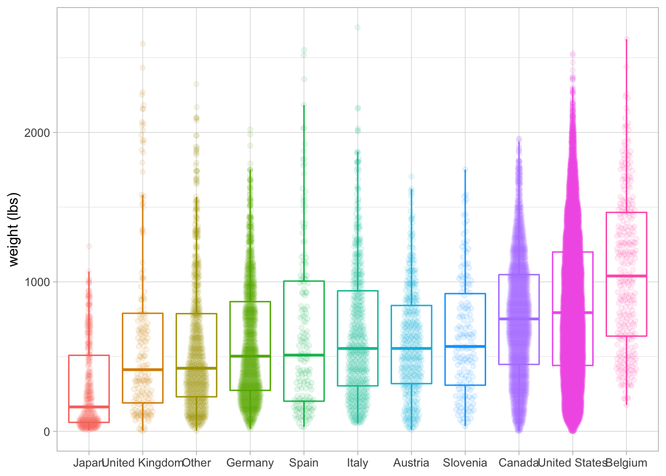
library(ggbeeswarm)
pumpkins %>%
  mutate(
    country = fct_lump(country, n = 10),
    country = fct_reorder(country, weight_lbs)
  ) %>%
  ggplot(aes(country, weight_lbs, color = country)) +
  geom_boxplot(outlier.colour = NA) +
  geom_quasirandom(alpha=0.1, width=0.2) +
  labs(x = NULL, y = "weight (lbs)") +
theme(legend.position = "none")Already added to the schedule!
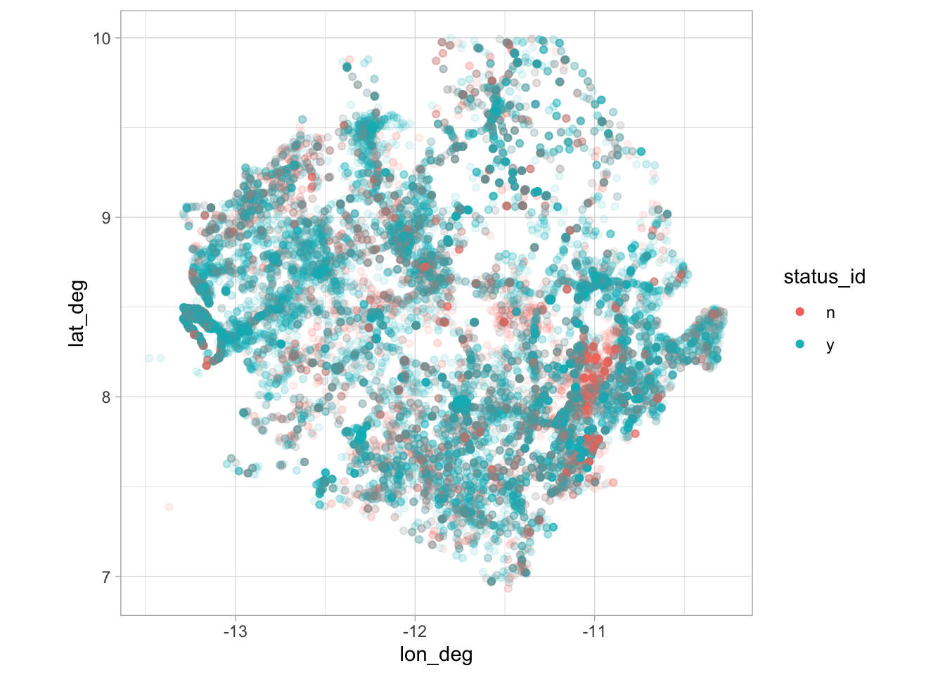
water_raw %>%
  filter(
    country_name == "Sierra Leone",
    lat_deg > 0, lat_deg < 15, lon_deg < 0,
    status_id %in% c("y", "n")
  ) %>%
  ggplot(aes(lon_deg, lat_deg, color = status_id)) +
  geom_point(alpha = 0.1) +
  coord_fixed() +
guides(color = guide_legend(override.aes = list(alpha = 1)))Already added to the schedule!
library(janitor)
library(tidyverse)
library(hrbrthemes)
library(viridis)
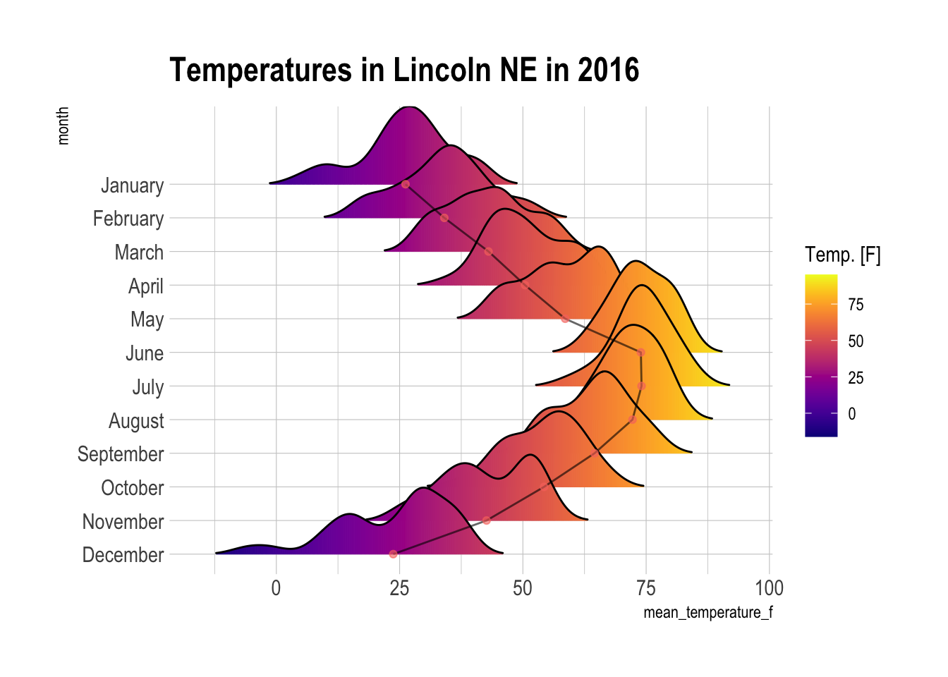
library(ggridges)
lincoln_weather %>%
clean_names() %>%
ggplot() +
geom_density_ridges_gradient(aes(x = `mean_temperature_f`, y = `month`, fill = ..x..),
scale = 3, rel_min_height = 0.01, alpha = 0.5) +
stat_summary(aes(x=mean_temperature_f, y = month, group=1),
geom = "line", alpha=0.6, fun=mean) +
stat_summary(aes(x=mean_temperature_f, y = month, color="#24EA53"),
geom = "point", alpha=0.6, fun=mean) +
scale_fill_viridis(name = "Temp. [F]", option = "C") +
scale_colour_discrete(guide = FALSE) +
labs(title = 'Temperatures in Lincoln NE in 2016') +
theme_ipsum() +
theme(
panel.spacing = unit(0.1, "lines"),
strip.text.x = element_text(size = 8)
)Already added to the schedule!
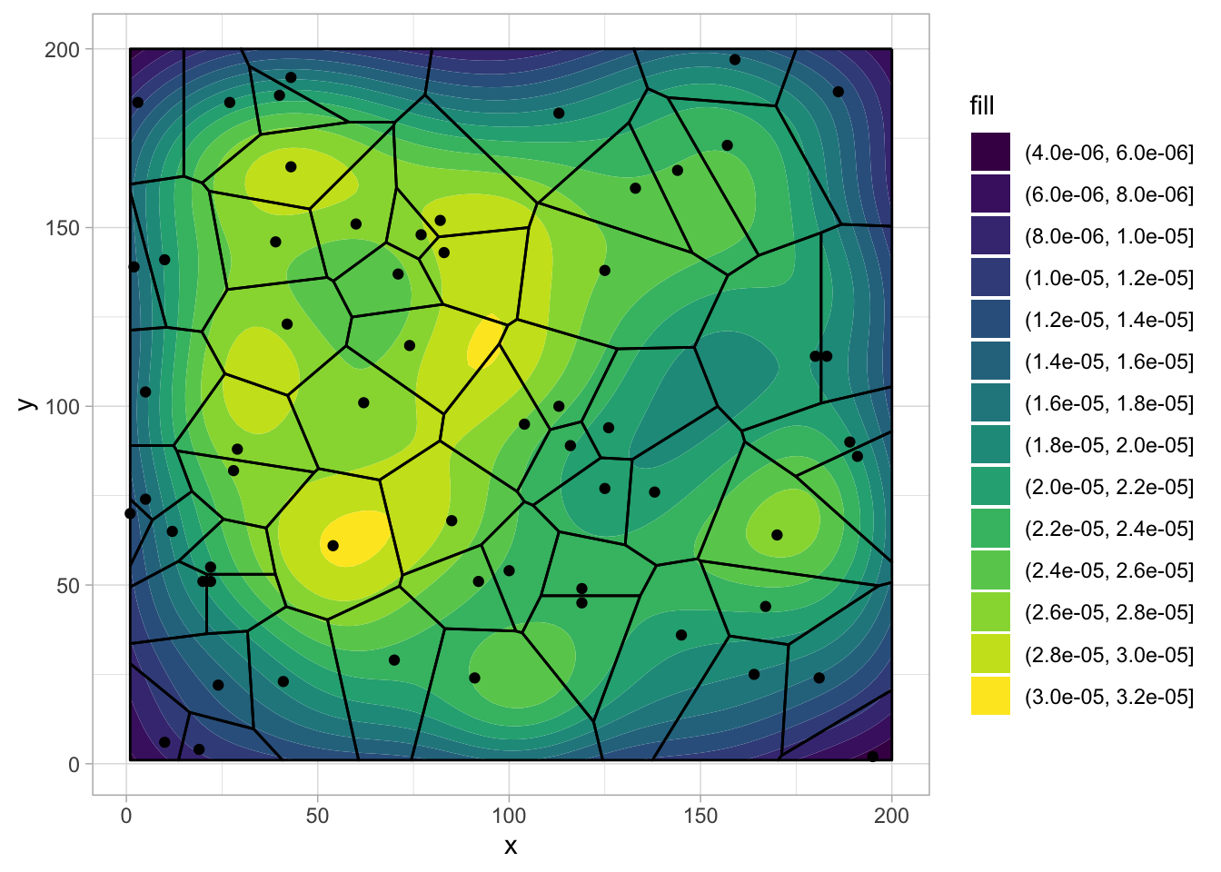
set.seed(2020)

ll <- rep(c(1:200),11)
square <- data.frame(x = c(1,200,200,1,1), y = c(1,1,200,200,1))
df_density <- data.frame(x=sample(ll, size = 500),y=sample(ll, size = 500))
df_point <- data.frame(x=sample(ll, size = 60),y=sample(ll, size = 60))
ggplot(df_point,aes(x,y)) +
  geom_density_2d_filled(data=df_density, aes(x,y)) +
  stat_voronoi(geom="path", outline = square) +
  geom_point() +
scale_fill_viridis_d()Already added to the schedule!
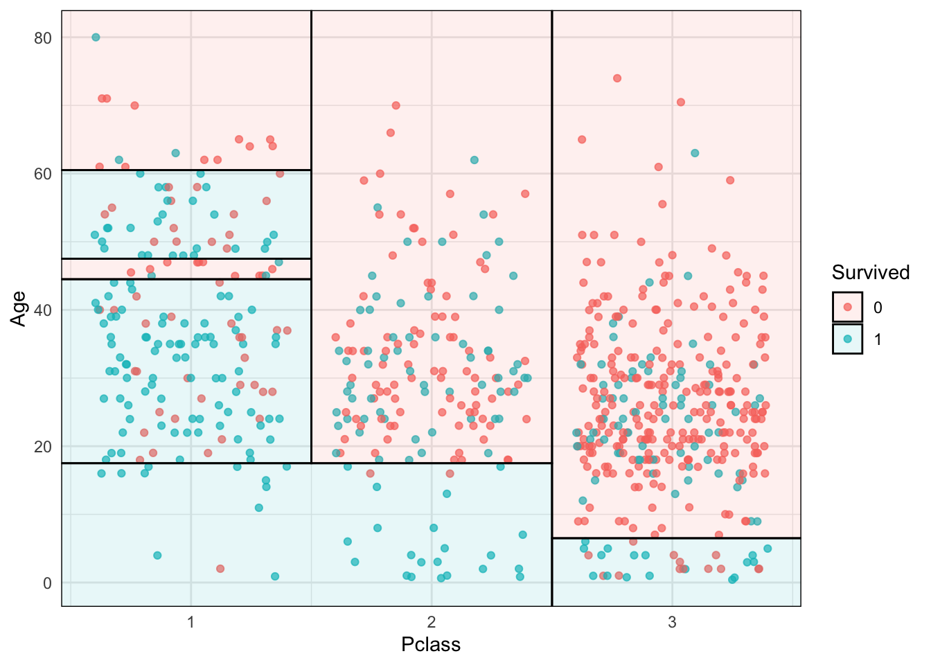
library("parsnip")
library("titanic") ## Just for a different data set
set.seed(123) ## For consistent jitter

titanic_train$Survived = as.factor(titanic_train$Survived)

## Build our tree using parsnip (but with rpart as the model engine)
ti_tree <-
  decision_tree() %>%
  set_engine("rpart") %>%
  set_mode("classification") %>%
  fit(Survived ~ Pclass + Age, data = titanic_train)

## Plot the data and model partitions
titanic_train %>%
  na.omit() %>%
  ggplot(aes(x=Pclass, y=Age)) +
  geom_jitter(aes(col=Survived), alpha=0.7) +
  geom_parttree(data = ti_tree, aes(fill=Survived), alpha = 0.1) +
theme_minimal()Already added to the schedule!
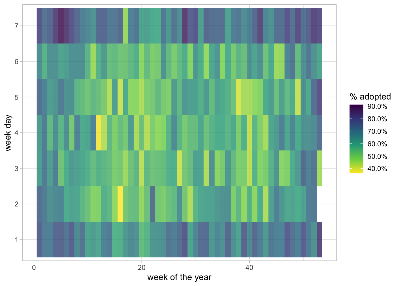
library(tidyverse)
library(lubridate)
library(scales)

train_raw <- read_csv("/train.csv")
# dataset available here: https://www.kaggle.com/c/sliced-s01e10-playoffs-2/
train_raw %>%
  mutate(outcome_type = outcome_type == "adoption") %>%
  group_by(
    week = week(datetime),
    wday = wday(datetime)
  ) %>%
  summarise(outcome_type = mean(outcome_type),.groups = "drop") %>%
  ggplot(aes(week, factor(wday), fill = outcome_type)) +
  geom_tile(alpha = 0.8) +
  scale_fill_viridis_c(labels = scales::percent, direction=-1) +
labs(fill = "% adopted", x = "week of the year", y = "week day")Already added to the schedule!
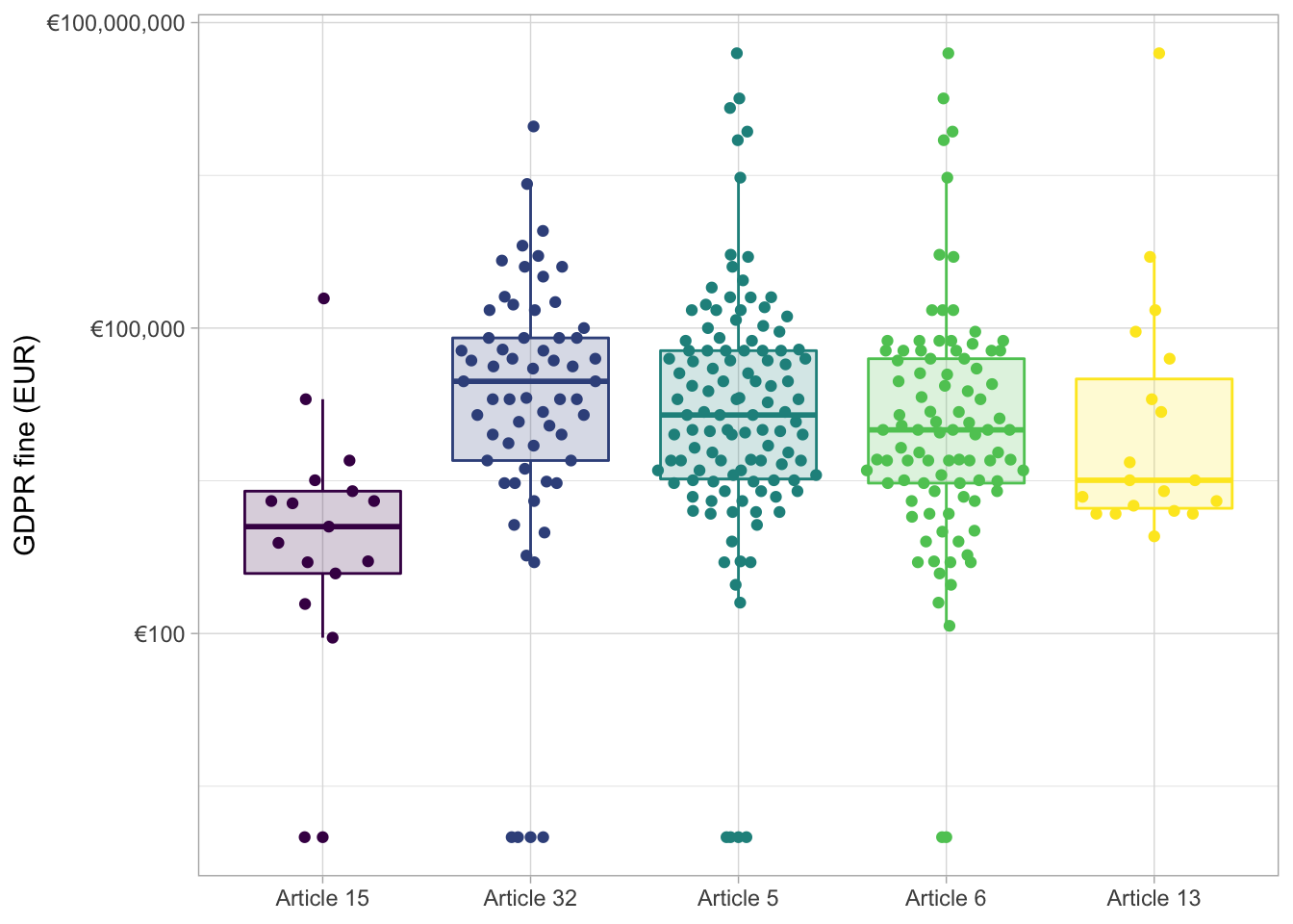
library(ggbeeswarm)
gdpr_raw <- readr::read_tsv("https://raw.githubusercontent.com/rfordatascience/tidytuesday/master/data/2020/2020-04-21/gdpr_violations.tsv")

gdpr_tidy <- gdpr_raw %>%
  transmute(id,
    price,
    country = name,
    article_violated,
    articles = str_extract_all(article_violated,
                               "Art.[:digit:]+|Art. [:digit:]+")) %>%
  mutate(total_articles = map_int(articles, length)) %>%
  unnest(articles) %>%
  add_count(articles) %>%
  filter(n > 10) %>%
  select(-n)

gdpr_tidy %>%
  mutate(articles = str_replace_all(articles, "Art. ", "Article "),
         articles = fct_reorder(articles, price, mean)) %>%
  ggplot(aes(articles, price + 1, color = articles, fill = articles)) +
  geom_boxplot(alpha = 0.2, outlier.colour = NA) +
  geom_quasirandom() +
  scale_y_log10(labels = scales::dollar_format(prefix = "€")) +
  labs(x = NULL, y = "GDPR fine (EUR)") +
  scale_fill_viridis_d() +
  scale_color_viridis_d() +
  theme(legend.position = "none")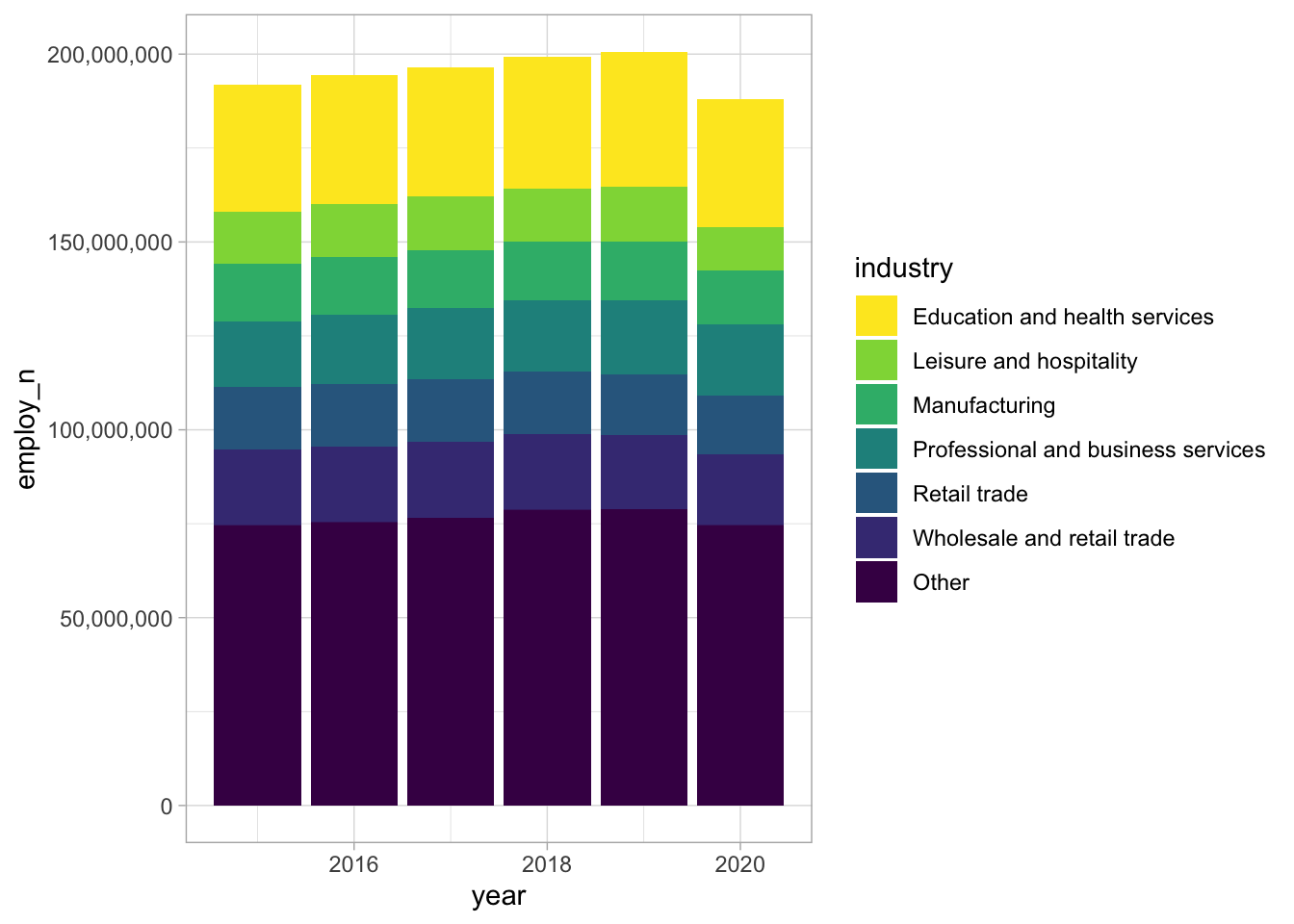
library(tidytuesdayR)

tt <- tt_load("2021-02-23")
tt$employed %>%
  mutate(dimension = case_when(
    race_gender == "TOTAL" ~ "Total",
    race_gender %in% c("Men", "Women") ~ "Gender",
    TRUE ~ "Race"
  )) %>%
  filter(dimension == "Total") %>%
  filter(!is.na(employ_n)) %>%
  mutate(industry = fct_lump(industry, 6, w = employ_n)) %>%
  ggplot(aes(x=year, y=employ_n, fill = industry)) +
  geom_bar(stat="identity") +
  scale_y_continuous(labels=comma) +
scale_fill_viridis_d(direction = -1)Already added to the schedule!
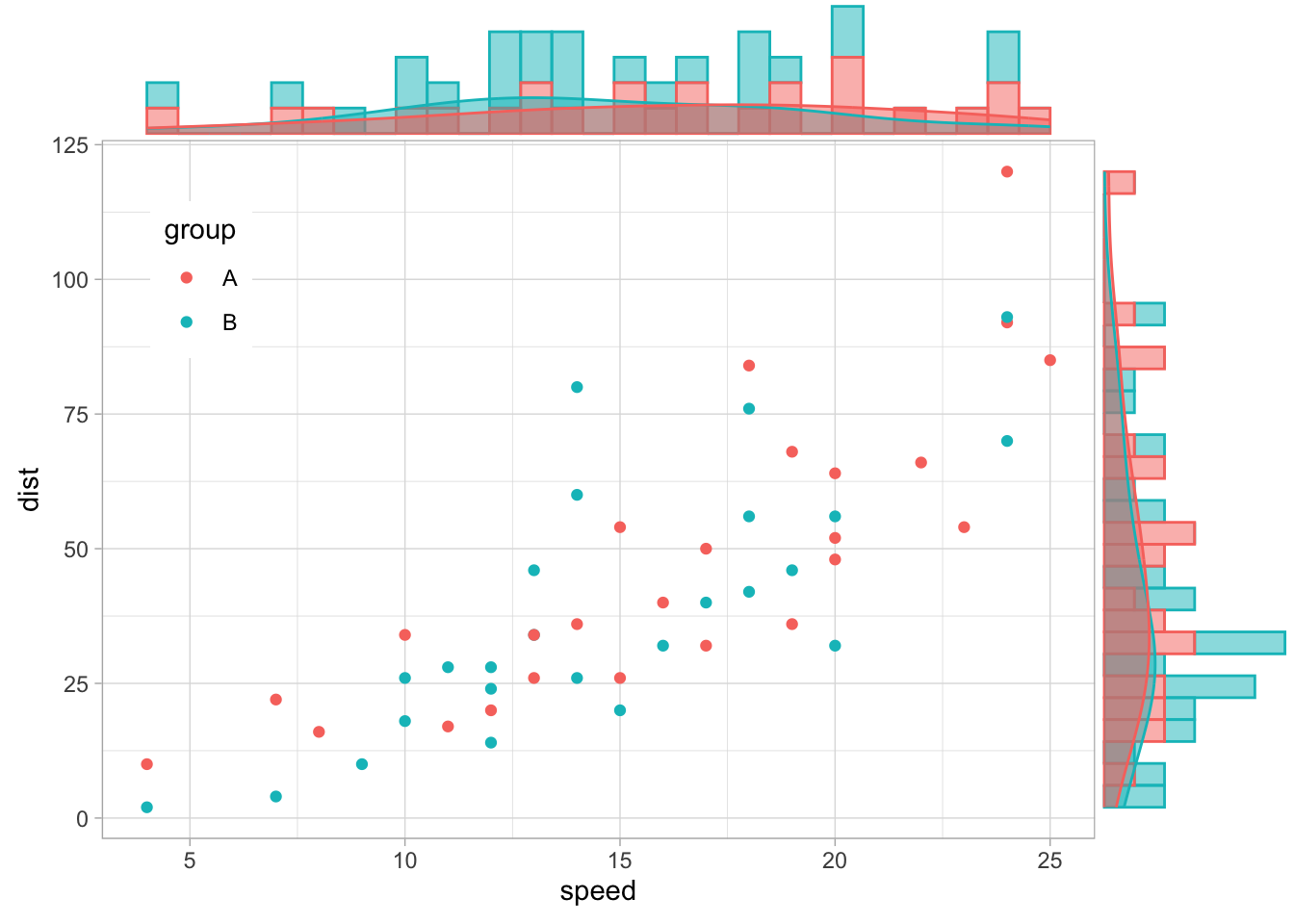
library(ggExtra)
cars$group <- c(rep("A", 25), rep("B",25)) %>% sample()

p <- ggplot(cars, aes(x = speed, y = dist, color = group)) +
  geom_point()+
  theme(legend.position = c(0.1,0.8))

# Densigram
ggMarginal(p, type = "densigram",
           groupFill = TRUE,
           groupColour = TRUE,
alpha = 0.5) Already added to the schedule!
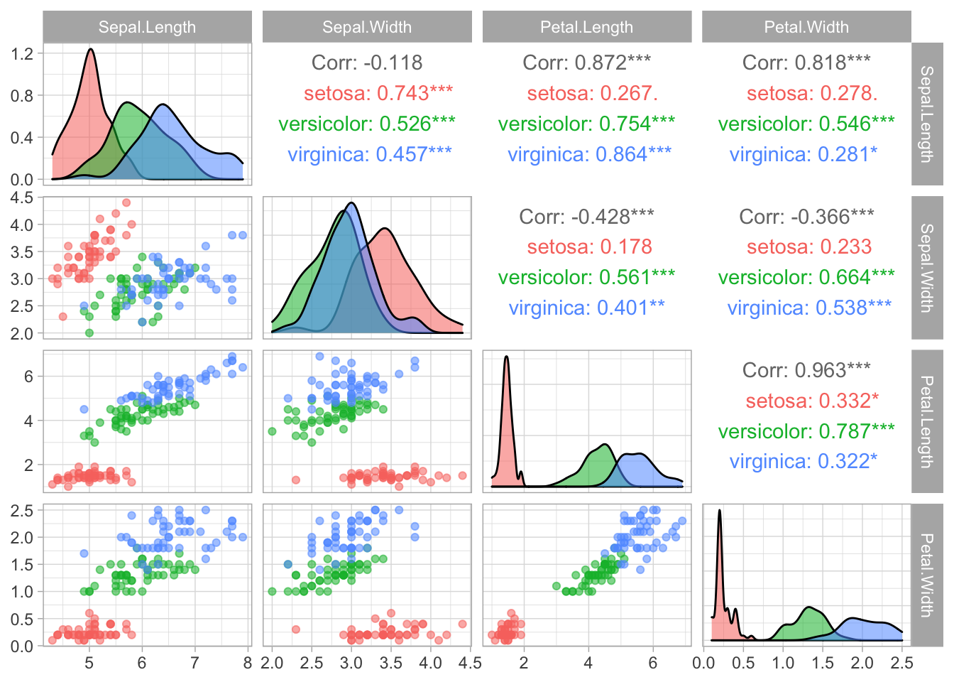
library(GGally)

ggpairs(iris, columns = 1:4, aes(color = Species, alpha = 0.5))Already added to the schedule!
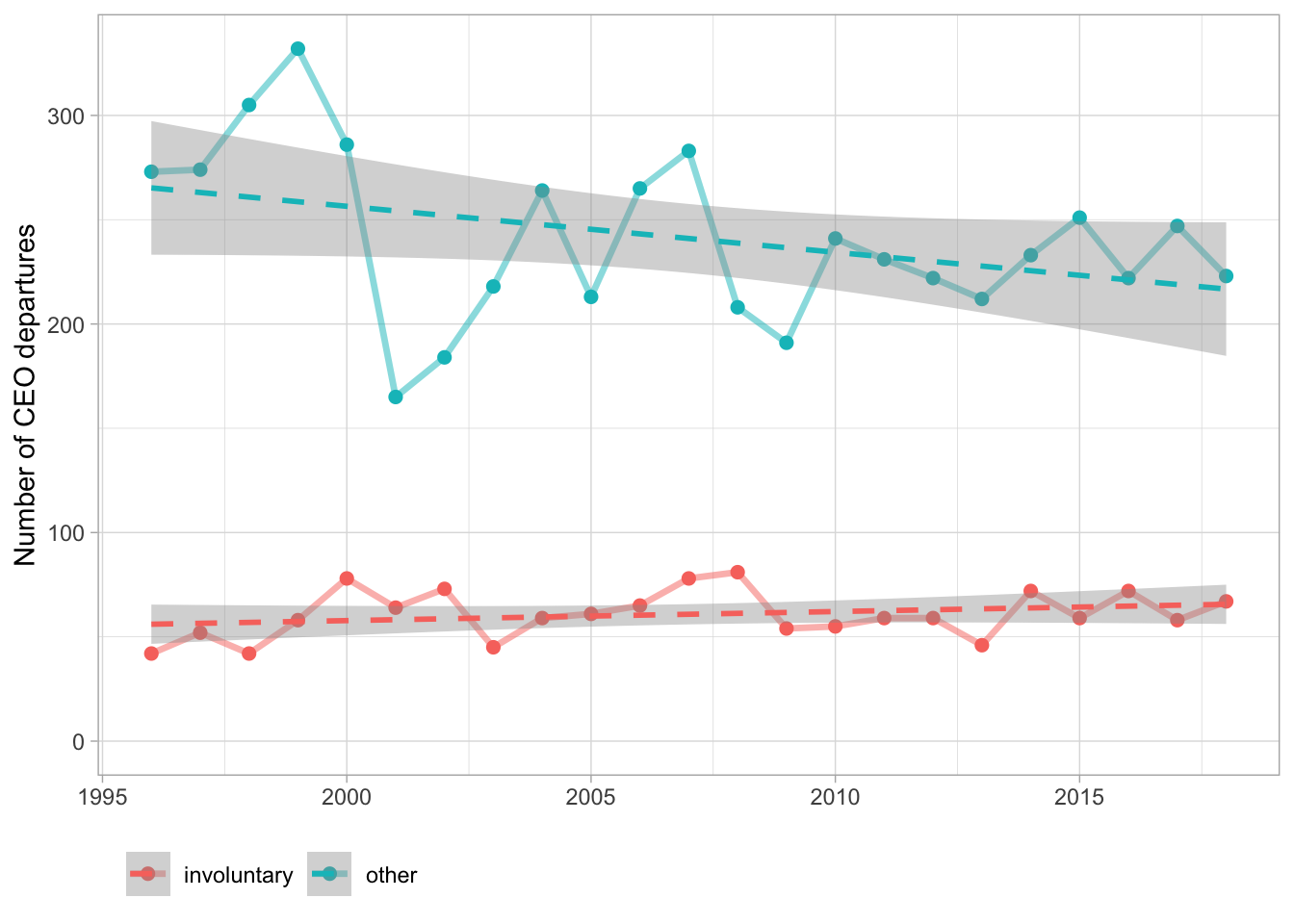
departures_raw <- read_csv("https://raw.githubusercontent.com/rfordatascience/tidytuesday/master/data/2021/2021-04-27/departures.csv")

departures_raw %>%
  filter(departure_code < 9) %>%
  mutate(involuntary = if_else(departure_code %in% 3:4, "involuntary", "other")) %>%
  filter(fyear > 1995, fyear < 2019) %>%
  count(fyear, involuntary) %>%
  ggplot(aes(fyear, n, color = involuntary)) +
  geom_line(size = 1.2, alpha = 0.5) +
  geom_point(size = 2) +
  geom_smooth(method = "lm", lty = 2) +
  scale_y_continuous(limits = c(0, NA)) +
  labs(x = NULL, y = "Number of CEO departures", color = NULL) +
  theme(legend.position = "bottom",
legend.justification = "left") Already added to the schedule!
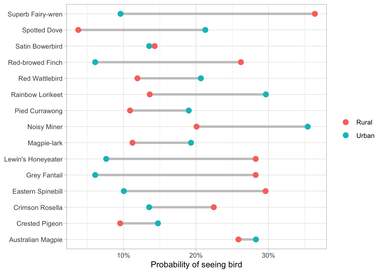
bird_baths <- readr::read_csv("https://raw.githubusercontent.com/rfordatascience/tidytuesday/master/data/2021/2021-08-31/bird_baths.csv")

top_birds <-
  bird_baths %>%
  filter(is.na(urban_rural)) %>%
  arrange(-bird_count) %>%
  slice_max(bird_count, n = 15) %>%
  pull(bird_type)

bird_parsed <-
  bird_baths %>%
  filter(
    !is.na(urban_rural),
    bird_type %in% top_birds
  ) %>%
  group_by(urban_rural, bird_type) %>%
  summarise(bird_count = mean(bird_count), .groups = "drop")


bird_parsed %>%
  ggplot(aes(bird_count, bird_type)) +
  geom_segment(
    data = bird_parsed %>%
      pivot_wider(
        names_from = urban_rural,
        values_from = bird_count),
    aes(x = Rural, xend = Urban, y = bird_type, yend = bird_type),
    alpha = 0.7, color = "gray70", size = 1.5) +
  geom_point(aes(color = urban_rural), size = 3) +
  scale_x_continuous(labels = scales::percent) +
labs(x = "Probability of seeing bird", y = NULL, color = NULL){{ template “_internal/disqus.html” . }}
To be continued…
Yu Cao
I am passionate about leveraging large language models for multimodal learning, with a specific focus on unsupervised domain adaptation and domain generalization.